Autocorrelation
Sources: ApX Machine Learning (2026a), Aghili (2023)
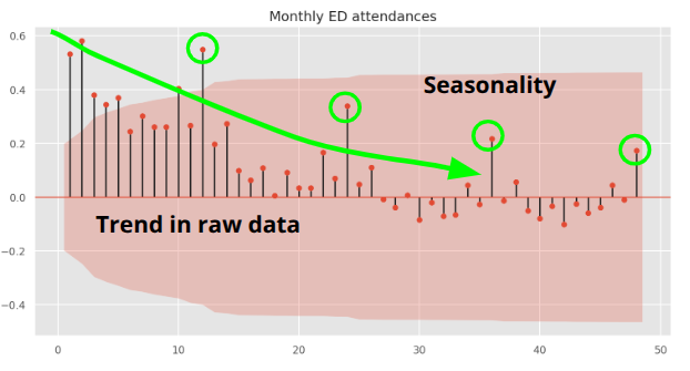
Autocorrelation is the correlation between observations within a time series, measured using the autocorrelation function (ACF). It calculates how correlated a series is with lagged versions of itself, comparing each value to the one one step before, then two steps before, three steps before, and so on.
For each lag, the ACF produces a single correlation coefficient between +1 and -1. On an ACF plot:
- X-axis is the lag (1, 2, 3…).
- Y-axis is the correlation coefficient for that lag.
A spike above the significance boundary indicates a meaningful correlation. For example, for daily data, a spike at lag 7 indicates weekly seasonality. For monthly data, a spike at lag 12 would indicate yearly seasonality.
Stationarity
Sources: Monks (2020), Hyndman and Athanasopoulos (2021b), Kim (2021)
A stationary time series has no predictable long-term pattern. It has:
- No trend… stable mean.
- No seasonality.
- Stable variance (the spread of values is stable and doesn’t grow or shrink over time).
Common methods of testing whether a time series is stationary are:
- Augmented Dickey Fuller(ADF) Test
- Phillips-Perron(PP) Test
- Kwiatkowski-Phillips-Schmidt-Shin(KPSS) Test
- Graphing rolling statistics such as mean, standard deviation
We can pre-process a time series to achieve stationarity. Common techniques include:
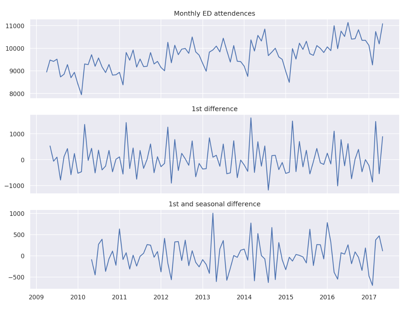
Differencing: Taking the first difference means subtracting each observation from the one before it. This removes a trend by focusing on the change between consecutive points rather than their absolute level.
Seasonal differencing: If the series looks seasonal, subtract observations a full seasonal period apart (e.g., subtracting the value from 12 months earlier removes a yearly pattern in monthly data).
Transformations: Mathematical transformations are used to simplify the patterns in historical data to make forecasting simpler and more accurate. Any forecasts are produced on a transformed scale, so the data then has to be back-transformed.
- If variances increases or decreases over time, a logarithmic transformation is often useful, since it stablising variance by compressing large values more than small ones. Although, it cannot be used if the time series contains zeroes or negative numbers.
Example:
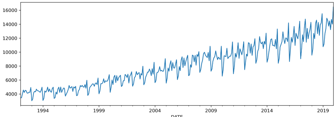
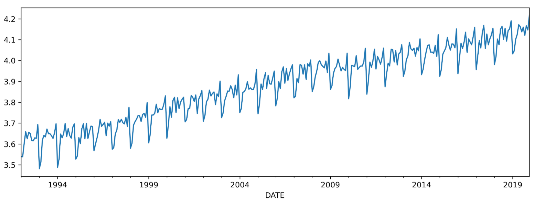
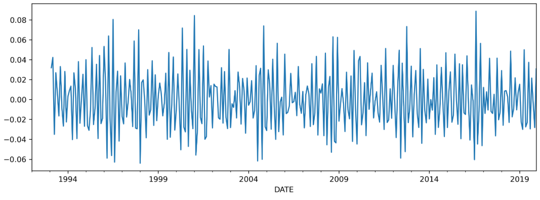
Now it is stationary! Can also inspect ACF afterwards too.
ARIMA
What is ARIMA?
Sources: Monks (2020), Kim (2021)
AutoRegressive Integrated Moving Average (ARIMA) (or “Box-Jenkins models”) is one of the most widely used forecasting techniques.
- AR - AutoRegressive: Predicts the current value using the series’ own past values (lags). It works like a normal regression, except the “predictor variables” are just earlier points in the same series instead of separate variables. For example, predicting this month’s demand using demand from the last 2 months.
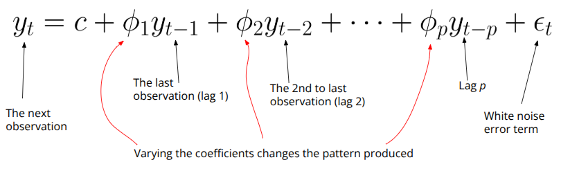
- I - Integrated: Refers to differencing the series to make it stationary.
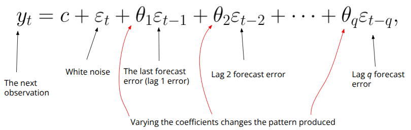
- MA - Moving Average: Predicts the current value using past forecast errors rather than past values. A forecast error is the gap between what the model predicted and what actually happened. If the model consistently underestimated demand last month, that error tells us something about the current month too. MA terms let the model “correct itself” using these recent misses, rather than raw past values.
Put together, ARIMA fits an AR and MA model to a differenced (stationary) version of the series, then reverses the differencing to produce forecasts on the original scale.
ARIMA assumptions
Sources: Monks (2020), Kim (2021)
ARIMA assumes data have:
- No seasonality - if there is, we should use Seasonal ARIMA (SARIMA) instead.
- No structural irregularities - for example, sudden one-off shocks like a policy change or COVID-19 lockdown, that aren’t part of the series normal pattern. ARIMA assumes that statistical relationship in the data stay consistent over time.
ARIMA parameters
Sources: Monks (2020), Kim (2021)
It has three parameters, often written as ARIMA(p,d,q):
| Parameter | Full name | What it controls |
|---|---|---|
| p | Order of AR term | How many past values (lags) of the series to use as predictors - e.g., to predict June, how many previous months’ data to include |
| d | Degree of differencing | How many times to difference the series to make it stationary. Usually d=1 is enough, but strong trends may need d=2. |
| q | Order of MA term | ow many past forecast errors to include as predictors |
Examples:
ARIMA(2,1,1) means we difference the data once (d=1), then predict using the last 2 values (p=2) and the last 1 forecast error (q=1).
ARIMA(1,0,2) means there is no differencing (d=0), then predict using the last value (p=1) and last 2 forecast errors (q=2).
ARIMA(1,1,0) means we difference the data once (d=1), then predict using the last value (p=2), and no MA terms are included.
Seasonal ARIMA (SARIMA)
Sources: Monks (2020), Hyndman and Athanasopoulos (2021a), Brenndoerfer (2025)
A seasonal ARIMA model adds extra terms to handle seasonality. It is written as:
ARIMA(p,d,q)(P,D,Q,m).
- (p,d,q) are the non-seasonal terms, same as regular ARIMA.
- (P,D,Q) are the seasonal equivalents.
- m is the seasonal period (e.g., 12 for monthly data with yearly seasonality, 7 for daily data with weekly seasonality).
The seasonal terms work the same way as the non-seasonal ones, just applied at seasonal lags (multiples of m) instead of consecutive lags:
| Component | Non-seasonal | Seasonal |
|---|---|---|
| AR terms | p: Based on recent timepoints (e.g., this month vs. last month, the month before). | P: Based on the same timepoint in previous seasons (e.g., this December vs. last December, the one before). |
| Differencing | d: Difference between consecutive observations, removes trend (e.g., December 2025 minus November 2025). | D: Difference between observations one seasonal period apart, removes seasonality (e.g., December 2025 minus December 2024). |
| MA terms | q: Based on recent forecast errors. | Q: Based on the forecast error at the same point in previous seasons. |
Example: SARIMA(2,1,0)(0,1,1,12) with monthly data.
p=2: This month depends on previous two months.d=1: One round of differencing to remove trend.q=0: No non-seasonal MA terms.P=0: No seasonal AR terms.D=1: One round of seasonal differencing.Q=1: This month’s forecast error depends on the forecast error from the same month last year.m=12: Yearly seasonality.
Order selection
Order selection and autoARIMA
Sources: Monks (2020), ApX Machine Learning (2026c)
Choosing the right values for ARIMA’s model parameters is called order selection, and it’s a key step in building a model that fits your data well. The order of a term is simply the number attached to it (e.g., an AR order of 2 means using the last 2 lags as predictors).
Traditional methods involve interpreting ACF and partial ACF (PACF) plots by eye. This approach doesn’t scale well though; manually inspecting plots for hundreds of time series or without training quickly becomes impractical.
The modern approach is to use the Hyndman-Khandakar algorithm, commonly known as autoARIMA. There are multiple implementations in Python and R. It systematically searches through combinations of p, d and q, fitting each candidate model and selecting the best one using the Akaike Information Criterion (AIC).
Akaike Information Criterion (AIC)
Sources: Monks (2020), ApX Machine Learning (2026b)
AIC is a metric used to compare candidate models. It balances two things:
- Model fit - how well the model explains the data.
- Model complexity - how many parameters the model uses.
AIC penalises models with more parameters, favouring simpler ones unless added complexity meaningfully improves fit. This helps avoid overfitting, where a model captures noise rather than genuine patterns.
The goal is to minimise AIC. Values are only meaningful in relative terms: a single AIC tells you nothing alone, but comparing values across models fitted to the same dataset shows which fits best.
Issues when using ARIMA in practice
Special calendar events
Sources: Monks (2020), Perplexity.
In ARIMA, differencing is great for smooth gradual repeated patterns like “Mondays are always busier” or “December is always slower”. It’s not well suited for sudden one-off jumps on a single date, even if that date happens every year. The spike size usually isn’t constant from year to year, you’d need many years of data to estimate it reliably, and leap years shift the calendar so “the same date” doesn’t always fall the same number of days apart.
If we don’t handle special calendar events explicitly, they distort the model’s understanding of normal day-to-day behavior. It might think the pattern is more volatile than it really is, or misjudge how quickly things bounce back after a busy day. By explicitly flagging an event like New Year’s Day as its own separate effect, the model can be more accurate for the holiday and the everyday pattern.
We handle this using regression with ARIMA errors. The regression predicts the outcome based on whether or not it’s New Year’s Day. The error from that regression, whatever’s left over and not explained by the New Year’s Day flag, is the remaining time series. ARIMA is then fit to that remaining error series, capturing the ordinary day-to-day pattern once the holiday effect has been accounted for separately.
All Python implementations can handle this for you, you just need to include a binary column marking the date.
Multiple seasonal periods
Sources: Monks (2020), Perplexity.
ARIMA only handles one seasonal period at a time, but data often has more than one seasonal pattern simultaneously. For example, daily data often has weekly seasonality (day-of-the-week) and yearly seasonality (month-to-month).
Two common ways to handle this, again using regression with ARIMA errors as extra regressors:
Dummy variables: Binary indicators for each category, e.g., one variable per month (11 dummies, since one month is the baseline) and one per weekday (6 dummies).
Fourier terms: Pairs of sine and cosine waves that can flexibly represent any repeating pattern’s frequency, rather than needing a separate dummy for every day or month. You choose how many sine/cosine pairs to include, trading off flexibility against overfitting.
However, this can become difficult to manage, and alternative methods like Prophet are often more practical.
Dynamic regression with lagged predictors
Sources: Hyndman and Athanasopoulos (2021a), Monks (2020), Perplexity.
The calendar-event examples above only flag the current day, e.g., “is today New Year’s Day.” But some effects linger beyond the day itself, New Year’s Eve celebrations might cause extra ambulance calls not just that night, but the next morning or two days later. A model checking only “is today New Year’s Day” would miss these delayed calls.
Dynamic regression with lagged predictors fixes this by adding lagged versions of the flag as extra regressors: alongside “is today New Year’s Day,” you add “was yesterday” and “was two days ago.” Each is checked against today’s call count, asking how much each past day still explains about today.
You test a few lag lengths (same-day only, +1 day, +2 days), fit a model for each, and pick whichever gives the lowest AICc (corrected AIC, corrects for small-sample bias). Whatever’s left over is still modeled with ARIMA as usual.