Current model
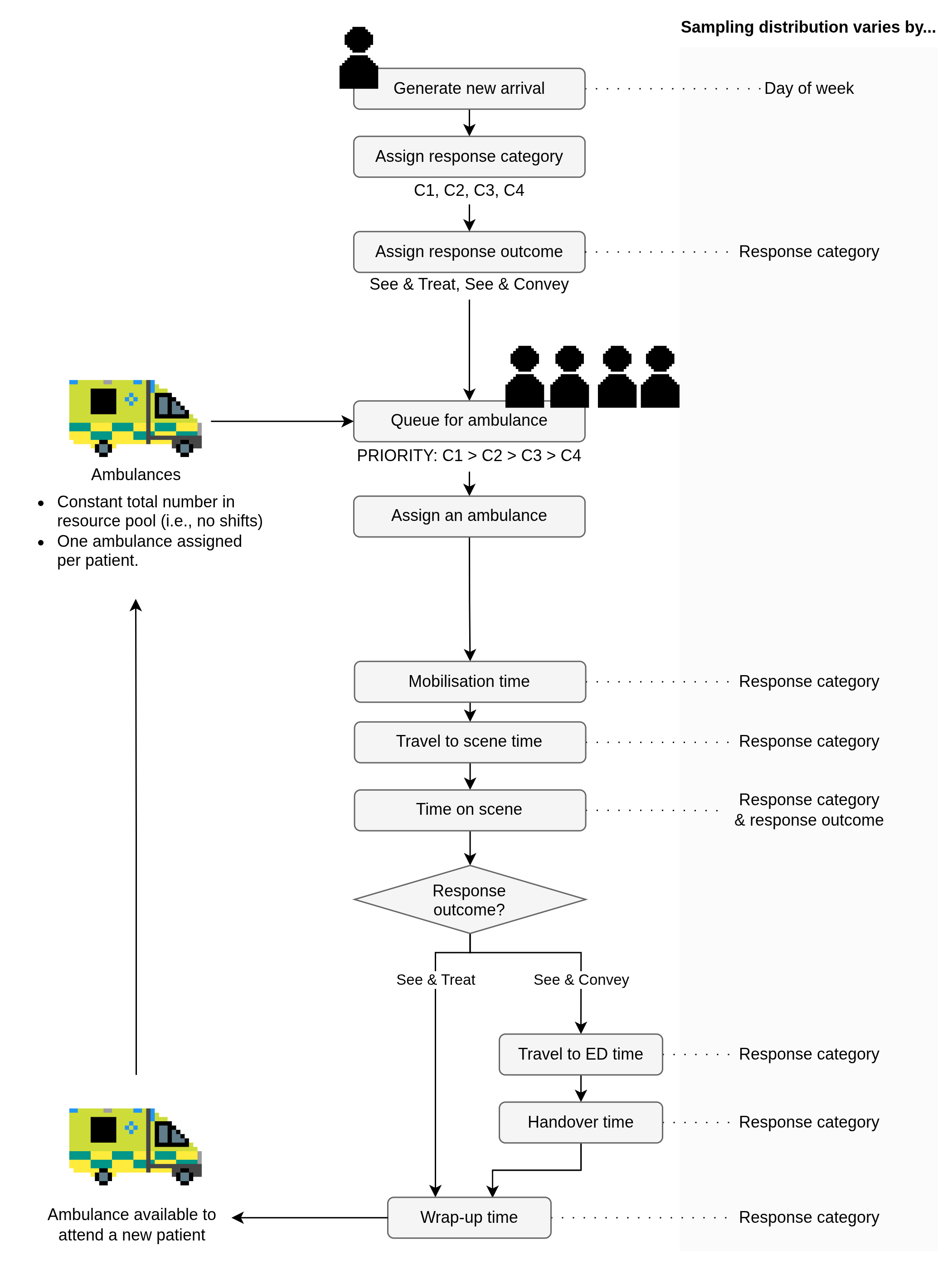
How can the model be used?
The model can answer the question:
How do changes in total vehicle hours, number of incidents per day, and/or handover delays affect Category 2 mean response time and resource utilisation?
We hope it can run quick enough to allow easy experimentation and scenario analysis. For example, it should be possible to ask: “If overall resource level changes by X hours, what happens to mean Category 2 response time?”
The main uses are resourcing and demand scenarios. Less commonly, scenarios involving:
Handover delays - these are difficult to predict, so can instead test scenarios like “What would happen if mean handover time was 60 minutes per patient.”
On-scene time - for example, “What would be the effect of reducing on-scene time by one minute?”
The model can represent the whole trust or an individual county. Historically, demand planning was undertaken at trust level, but there has been a move to do county-level too in recent years. Counties may have the same targets as each other, or maybe different targets (e.g., one county aiming to reduce job cycle by X minutes, another by Y minutes).
The model structure is consistent across areas - only the input files change. Running separate county models is equivalent to modelling one trust-wide system with separate ambulance resource pools for each county and no interaction between them. Running separate single-area models is therefore simpler.
Comparison with the regression models
The DES should broadly agree with estimates from the existing regression models, while offering richer outputs. Regression is simpler, faster and easier to validate. However benefits of DES are:
- Multiple outcomes from a single run, whereas regression produces one outcome per model.
- A more intuitive representation of the system, showing how resourcing assumptions translate into waits and utilisation.
- More scope for extension.
The current regression model changes three inputs:
- Vehicle hours
- Number of incidents per day
- Handover delays
Validation is important at both trust and county level. Something that is bad at a trust level could look good at a county level and vice versa.
Assumptions
Definition: Assumptions arise from incomplete knowledge - you do not know exactly how something works, so you use the best available information.
You can also identify simplifying assumptions. These are assumptions that lead to simplification of the model. (Robinson and Brooks (2025))
Robinson and Brooks (2025) recommend assessing:
- Confidence - how certain we are that the assumption is correct.
- Impact - the anticipated effect on outputs if the assumption is incorrect - independent of the likelihood of the assumption being correct.
They recommend that sensitivity analysis can be used to measure the impact of changing an assumption.
| Assumption | Confidence | Impact |
|---|---|---|
Extreme values: Values above the 99.9th percentile are treated as missing (NA), on the assumption that they are more likely to reflect data quality issues than genuine operational times. |
High: The data were discussed with system experts who agreed that very long times are often caused by data-quality issues, but said it’s hard to draw a definitive threshold | Low: Extreme values can make distribution fitting a little harder as it distorts visualisations. However, fitting with and without these values actually had relatively minimal impact on the selected distributions or model outputs. |
| NHPP arrivals: Arrivals are represented by an NHPP - a common approach for DES in the literature - assuming arrivals occur independently and follow a Poisson distribution, and vary over time. | Medium: NHPP is established practice for time-varying service demand arrivals and captures known variation in demand over time. However, marked as “medium” not “high” as not yet assessed independence, clustering and variability in arrivals. | Medium: If arrivals are more variable than NHPP allows or are correlated or clustered, then the model may understate the variation in demand and risk of extreme demand periods. |
| Process and activity durations: These are represented by probability distributions selected through input modelling. They are assumed to adequately represent the observed data. | High: Distributions and parameters were selected using input modelling and graphical and statistical measures of fit. | Low: Sensitivity testing using fitted distributions v.s., empirical sampling produced similar results, suggesting relatively minimal impact of using fitted distributions. |
Simplifications
Definition: Simplifications are a deliberate design choice - you could model something in more detail, but you opt for a simple representation. (Robinson and Brooks (2025))
Robinson and Brooks (2025) recommend assessing the impact of simplifications - i.e., it’s anticipated effect on model outputs.
| Simplifications | Impact |
|---|---|
| Arrival frequency: Arrival frequency varies by day of week. Response category and response outcome are assigned after arrival and do not change by day of week. | Low: The proportion of Category 1-4 incidents and of see-and-convey v.s., see-and-treat outcomes, was compared across days of the week and found to be consistent. If a clear day-of-week pattern was later identified, then the response category and outcome should be sampled as part of the NHPP rather than assigned afterwards. |
| Conveyance: “See & Convey non ED” and “See & Convey ED” are combined into a single “See & Convey” group. | Low: This level of aggregation matches the reporting level required by SWAST. |
| Queueing and dispatch: Queueing is represented by priority sorting, with no other behaviours (e.g., reneging, balking). Operational colleagues noted that, in reality, geography and queues within dispatch areas also affect dispatch decisions. | High: It is anticipated that the current queueing process is having a large impact on outcomes, causing very low C1/C2 times and very high C3/C4 times. |
| Special events: Events (e.g., festivals) have been removed from time data. | Low: This is typical for SWAST operational modelling. If we wanted to explore special events in the model, this could be performed via scenario analysis altering demand. |
| Vehicle types: All vehicle types are pooled and represented as one ambulance resource type. The model does not distinguish e.g., double-crewed ambulances, cars, community first responders, other specialist vehicles. | Medium: Vehicle types have different capabilities (e.g., conveyance v.s., not, or targeted at different job types), utilisation, job duration. Also, if a car attends a patient requiring conveyance, the clock stops when an ambulance arrivals, so recorded response time looks longer. |
| Sickness abstraction: Sickness is represented either as a fixed reduction in the resource pool or a daily sampled reduction. | Low: This simplification captures average loss of capacity. Used a fixed or daily sampled reduction produces similar results. |
| Staff-to-vehicle sickness conversion: Sickness data is provided as staff-hours per day. This is converted to vehicle-hours by halving the number of staff hours, without accounting for the mix of single- and double-crewed vehicles. | Medium: This conversion may over- or under-estimate the number of unavailable vehicles. |
| Resource availability over time: The model uses one resource pool. It doesn’t represent… (A) Shifts. These can vary alot hour-to-hour, day-to-day, day-v.s.-night, with differences up to even 100 resources. (B) Other abstractions besides sickness. (C) Restricted send during rest breaks or end of shift (this has a big impact on availability). (D) Any other issues or problems on shift. | High: There is alot of variability not represented, with large impact on resource numbers. |
| Resource availability by location: The model uses one resource pool, but resources are actually organised by dispatch areas. Dispatch areas are smaller than counties, and are areas where it is feasible to send ambulances. They were designed for operational use. Several are set up around acutes, but not all will include an acute. Resources in different areas have different response times. Even within the dispatch area, C3 near resource or C1 far from resource, will choose the C3, and instead have a non-core go to C1 or do call-out asking for resource. | Medium-to-high: Lots of impact on dispatch, not represented in model. |
| Multiple-resource incidents: In the model, each incident receives one ambulance resource. The average capacity used by additional resources at multi-resource incidents is represented by reducing the available ambulance pool by an estimated average amount (see Estimating the ambulance pool page). This is done instead of modelling multiple resources directly as that would require complex dispatch rules. If a lower-priority incident is waiting for a second ambulance when a higher-priority incident arrives, the model must decide which incident receives the next available ambulance. Also, all resources would need to arrive before the sampled on-scene time ends, which would be tricky to guarantee. | Medium: This approach represents the average extra capacity used by multi-resource incidents - but has some limitations… (A) Does not capture clusters of multi-resource incidents or short-term shortages caused by several occurring at once. (B) Assumes additional ambulances are occupied for the category-average job duration - but this is likely an overestimate if they arrive later, leave earlier, or do not convey the patient. |
| Hear-and-treat: Excluded. | Low: Agreed scope with SWAST is to exclude hear-and-treat. Hear-and-treat is assumed to not materially affect dispatched ambulance activity. |
| Out-of-area activity: Activity outside of SWAST and across county boundaries is not represented. | Medium: Although the model doesn’t capture interactions between counties (e.g., where patients are frequently conveyed out of their originating county), this simplification may be acceptable. The model groups activity by location where the call is received, rather than by the location of hospital attendance. As a result, it represents demand originating from each county, meaning that differences in response times driven by local demand and resource availability (e.g., longer response times in higher-pressure areas) are still reflected. |
| Times for see-and-treat v.s., see-and-convey: Separate distributions for time on scene, but otherwise use a single distribution. | Medium: This is based on discussion with system experts, who identified time on scene as necessary to model separately. This could be reduced to “low” if checked data to see other times don’t vary markedly. |
| Upgrading and downgrading: Provided data just has final category decision for each patient. In reality, some category 1 might downgrade to category 2 and so on. Also, like after X time, welfare call to check in, and maybe then change e.g., C3 to C2. Note, this will reset the clock. | Low: Assumed that category changes are relatively uncommon and therefore this should have a minimal impact. |
Other notes
Even in this simplest stage, we can’t just have one service time, as we need to be able to:
- Calculate response time output
- Input varying handover delay
SWASFT are normally interested in category 2 mean response time for a given day of the week (e.g., a Monday), or a given week or year. They don’t look within the day at response times by time of day. In which case, arguably not relevant to include time of day in NHPP. Their typical profile is:
- Higher activity at weekend.
- Longer handover delays on Mondays (as they’ve built up over weekend).
Therefore, we agreed it best to use NHPP by day of week.
We don’t explicitly ensure that time distributions are returning “zero”. Just very short times.