----------------------------------------------------------------------
This is the API documentation for the ambdes library.
----------------------------------------------------------------------
## Classes
Core classes
WarmUpAuditor(model, interval)
Warm-up auditor - records cumulative mean results at intervals.
Attributes
----------
model : Model
A model instance that has not yet been run (model.run()).
interval : int
Audit frequency in minutes.
audit_results : list
List of dictionaries containing audit snapshots at each interval.
response_categories : list
List of response categories.
SimConfig(arrivals_json, times_json, param_csv)
Configuration for a simulation run.
Stores input data and run settings used by the model.
Attributes
----------
dist_config : dict
Dictionary with all distribution settings, in required format for
sim-tools DistributionRegistry.
n_ambulances : int
Size of ambulance resource pool.
warm_up_period : int
Duration of the warm-up period in minutes.
data_collection_period : int
Duration of the data collection period in minutes.
n_reps : int
Number of replications to run.
cores : int
Number of CPU cores to use for parallel execution. To use all
available cores, set to -1. For sequential execution, set to 1.
FitDist(data, metric_name)
Fit distributions using sim-tools and compare samples to real data.
Attributes
----------
data : pd.Series
Time data to fit distribution to.
metric_name : str
Name of metric, used for plot titles.
mean : float
Mean of `data`.
stdev : float
Standard deviation of `data`.
min : float
Minimum value of `data`.
max : float
Maximum value of `data`.
mode : float
Mode of `data`. If there are several modes, it chooses the middle one.
Model(run_number, config)
Discrete-event simulation model for generating patient calls.
The model creates one call-generation process per patient category and
records generated patients during a single simulation run.
Patient(patient_id, category, outcome, call_timestamp)
Represents a patient who has called 999.
Attributes
----------
patient_id : int
Unique identifier for the patient.
category : str
Ambulance response category ("C1", "C2", "C3" or "C4").
outcome : str
Call outcome ("see_and_convey" or "see_and_treat").
call_timestamp : float
Time at which patient called 999.
wait_for_assignment : float
Time between the call and an ambulance being assigned.
response_time : float
Time between the call and ambulance arrival on scene.
Results(model)
Simulation output for a single model run.
UtilisationCalculator(log, warm_up_period, data_collection_period, capacity)
Compute time-weighted ambulance utilisation from an event log.
Attributes
----------
log : pd.DataFrame
Event log from a vidigi EventLogger.
warm_up_period : float
Length of the warm-up period - observations before this time are
excluded.
data_collection_period : float
Length of the data collection period.
run_length : float
Total run length (including warm-up and data collection period).
capacity : int
Total number of ambulances.
Runner(config)
Run the simulation for one or more replications.
## Functions
Public functions
plot_warm_up(audit, metric, category=None)
Plot warm-up trajectories for one metric and response category.
Shows one line per run for the cumulative mean trajectories, and overlays
the overall cumulative mean across runs.
Parameters
----------
audit : pd.DataFrame
Warm-up audit results.
metric: str
Name of the performance measure to visualise.
category : str
Response category to plot.
Returns
-------
fig : matplotlib.figure.Figure
A Matplotlib Figure containing cumulative mean trajectories for
each run and the overall cumulative mean.
ax : matplotlib.axes.Axes
The Matplotlib Axes object.
run_warm_up_audit(config, interval, n_reps)
Run warm-up audit for one or more replications (can run in parallel).
Parameters
----------
config : object
Configuration object containing model parameters.
interval : int
Audit frequency in minutes.
n_reps : int, optional
Number of replications to run.
Returns
-------
pd.DataFrame
Audit results with one row per run, time, category and metric.
build_arrival_config(arrivals)
Determine arrival parameters and create config dict.
Parameters
----------
arrivals : pd.DataFrame
Count of arrivals by weekday, response category and outcome.
Returns
-------
dict
Dictionary containing the configuration dictionary, as well as other
tables and outputs from processing, that can be used to help check
assumptions in the arrival modelling.
fit_config(time_data, time_data_unit, metric_config)
Fit distributions for each metric and category from raw time data.
If specified in `metric_config`, times may be additional split depending
on whether patients were conveyed (see & convey) or not (see & treat).
Parameters
----------
time_data : pd.DataFrame
Raw time data.
time_data_unit : str
Whether the provided raw data is in seconds ("s") or minutes ("m").
metric_config : dict
Dictionary where keys are the times, then sub dict, has dist sim-tools
name and column mapping to column in raw time data for that time.
Returns
-------
config : dict
Dictionary in format suitable for sim-tools distribution registry
with generated parameters for dists by category etc.
plot_metric_kde(metric, registry, size=10000)
Plot KDE curve by category (C1-C4).
Sample from the fitted distribution stored in the registry for the given
metric. Will split by conveyance status if nested.
Parameters
----------
metric : str
Name of metric to plot.
registry : simtools.distributions.DistributionRegistry
Registry instance set-up using the distribution config.
size : int
Number of samples to draw from each category's distribution.
plot_observed_fitted(data, sample, kind='hist', xmax=200, title='')
Plot overlaid comparison of observed vs fitted data.
Parameters
----------
data : array-like
Observed data values.
sample : array-like
Sampled/fitted distribution values.
kind : str
Either "kde" (density curve) or "hist" (plain count-based histogram).
xmax : int or None
X-axis limit for a second, optional cropped copy of the plot.
title : str
Title.
Returns
-------
fig : matplotlib.figure.Figure
Figure with two sets of overlaid histograms (one standard, one
cropped).
## Constants
Module-level constants and data
DISTRIBUTIONS
Built-in mutable sequence.
If no argument is given, the constructor creates a new empty list.
The argument must be an iterable if specified.
----------------------------------------------------------------------
This is the User Guide documentation for the package.
----------------------------------------------------------------------
### Assumptions and simplifications
As defined by [Robinson 2024](https://www.bloomsbury.com/uk/simulation-9781350445222/):
* **Assumption** - arises from incomplete knowledge - you do not know exactly how something works, so you use the best available information.
* **Simplification** - deliberate design choice - you could model something in more detail, but you opt for a simple representation.
## Assumptions
Rough notes!
* Times: Choices around cropping any times when input modelling (e.g., extreme values - 0 or very high).
* Arrivals...
* In the model, the number of arrivals vary by day of week.
* The arrivals are assigned a response category and a response outcome. These are assumed to not vary by day of week. We check this assumption by looking at the proportion on each day of the week of C1 v.s., C2 v.s., C3 v.s., C4 and likewise by see and convey v.s., see and treat.
## Simplifications
Rough notes!
* Grouped 'See & Convey non ED' and 'See & Convey ED' into a single 'see & convey' group.
* Queueing - simplified - priority sorting.
* They tend to take events out of the times data.
* Vehicles -
* Only one resource per patient - not multiple.
* Just one vehicle type - not multiple.
* Just one fixed pool of resources - no shifts and changes in availability across week.
* Arrivals - just vary by day of week.
* Excluding hear-and-treat.
* Excluding out-of-area activity.
### Best practice criteria
This page documents the best practice criteria we are aiming to adhere to across this work as part of our [quality assurance](qa.qmd).
We include the raw Markdown checklists that you can copy and adapt for your own projects, along with links to the corresponding GitHub issues for this project where progress against each checklist is tracked.
## STRESS-DES
STRESS-DES is a reporting checklist for discrete-event simulation studies. It helps ensure the model, data, assumptions, experimentation, and implementation are described clearly enough for others to **replicate** the work.
> **Replicable:** New code based on described methods produces consistent results. Gives confidence in results, their validity and reliability.
View progress
::: {.callout-note title="View blank checklist" collapse="true"}
```markdown
{{< include ../assets/checklists/stressdes.md >}}
```
:::
## STARS reproducibility recommendations
These recommendations focus on making simulations **reproducible**, derived from computational reproducibility assessments of published healthcare DES models.
> **Reproducible:** Running code regenerates the published results. Verifies code is working as expected and increases trust.
View progress
::: {.callout-note title="View blank checklist" collapse="true"}
```markdown
{{< include ../assets/checklists/stars_reproducibility.md >}}
```
:::
## STARS reuse framework
This framework focuses on making DES models more **reusable**.
> **Reusable:** Code can be adapted and used in next contexts. Saves time and increases impact.
View progress
::: {.callout-note title="View blank checklist" collapse="true"}
```markdown
{{< include ../assets/checklists/stars_reuse.md >}}
```
:::
## NHS Levels of RAP
This framework provides a staged path for NHS teams to implement RAPs into their analytical work.
View progress
::: {.callout-note title="View blank checklist" collapse="true"}
```markdown
{{< include ../assets/checklists/nhs_levels_of_rap.md >}}
```
:::
## DES RAP Book verification and validation checklist
This checklist translates verification and validation guidance from the simulation literature into concrete, practical steps to build confidence in DES models.
View progress
::: {.callout-note title="View blank checklist" collapse="true"}
```markdown
{{< include ../assets/checklists/vv.md >}}
```
:::
## HSMA model readiness checklist
This staged checklist provides guidance for deciding whether a DES model is ready enough to support real-world decision-making.
View progress
::: {.callout-note title="View blank checklist" collapse="true"}
```markdown
{{< include ../assets/checklists/hsma_model_readiness.md >}}
```
:::
## PyOpenSci package checks
PyOpenSci is a volunteer-led organisation that conducts peer review of scientific Python packages. Their review template is a curated checklist of best-practice criteria covering packaging, testing, documentation, and sustainability, which they apply when assessing packages.
View progress
::: {.callout-note title="View blank checklist" collapse="true"}
```markdown
{{< include ../assets/checklists/pyopensci.md >}}
```
:::
### Literature
This page summarises how **published ambulance DES** represent key elements of the ambulance system. It builds on the excellent review by @aboueljinane_review_2013, whose clear structure and introduction to ambulance DES have shaped how I organise the sections here. I include the DES from that review, and I have also read and added more recent ambulance DES models.
## Call arrival timing
In all DES studies, call arrivals are modeled using a **Poisson** process, so inter-arrival times are exponential. This is standard for arrival processes in healthcare DES models.
Some studies use a **Homogeneous Poisson process (HPP)** with a single arrival rate for the entire simulation period. However, most use a **Non-homogeneous Poisson process (NHPP)** where the arrival rate varies over time (e.g., by hour of day or day of week).
::: {.callout-note title="View studies" collapse="true"}
HPP:
* @silva_emergency_2010
* @van_buuren_evaluating_2012
NHPP by time of day only:
* @gigante_study_2022 - by period (00:00-08:00, 08:00-16:00, 16:00-00:00)
* @kergosien_generic_2015 - by 2-hour intervals
NHPP by time of day and day of week:
* @wei_lam_reducing_2014 - by 2-hour intervals and day of week
* @fonseca_discrete_2025 - by hour and weekday/weekend
* @aboueljinane_reducing_2012 - by hour and weekday/weekend
* @pinto_generic_2015 - by hour and day of week
* @wu_using_2009 - by hour, day of week and month
NHPP incorporating call location:
* @ingolfsson_simulation_2003 - by time of day, day of week and zone
* @maxwell_ambulance_2009 - by time of day and zone
* @berlin_mathematical_1974 - by node
* @wang_discrete-event_2025 - live data from Baidu Heatmap giving information on number of people in each grid, extracted on a hourly basis, to get representative data for each hour from Monday to Sunday
Trace-driven:
* @henderson_ambulance_2005
* @uyeno_practical_1984
* @wang_discrete-event_2025 (designed to allow it, but no current access, so reports sampling, as above)
:::
## Call location
Models differ in how they represent where call occur:
* Some do **nothing** to represent location.
* Some embed location in the **NHPP**, giving each zone its own arrival rate.
* Some generate calls first, then **assign each call to a zone** using a probability distribution, with that distribution sometimes time-varying.
@aboueljinane_review_2013 note that studies generally assume demand is located at the **centre** of the corresponding zone (though not always).
::: {.callout-note title="View studies" collapse="true"}
Do not represent call location:
* @fonseca_discrete_2025
NHPP incorporating call location (as above):
* @ingolfsson_simulation_2003
* @maxwell_ambulance_2009
* @berlin_mathematical_1974
* @wang_discrete-event_2025
Assign zones to generated calls:
* @wu_using_2009 - cluster historical calls into nodes using Nearest Neighbor Hierarchical clustering, then estimate probability a call comes from each node, and use that for a **multinomial distribution** sampling probability of each node.
* @gigante_study_2022 - calls are **evenly distributed** among the 4 regions
* @pinto_generic_2015 - city divided into cells, calls assigned using an **empirical discrete distribution** over cells that **varies by time of day and day of week**, and coordinates drawn randomly within the chosen cell.
* @kergosien_generic_2015
* Urgent calls: assign to zone using **discrete distribution** with probability proportional to demographic weight.
* Transfer calls: assigned to hospital (85%) or home (15%) - home coordinates drawn randomly.
* @wei_lam_reducing_2014 - call locations within each district sampled from an **empirical distribution** for each **4‑hour interval over the week**.
*Empirical is often used when data doesn't fit well to a distribution. An empirical distribution will divide the data into groups and calculate the probabilities of each.*
Unclear call location mechanism:
* @aboueljinane_reducing_2012
:::
In the studies, call location typically affects **travel times** - but can also influence resource dispatching, hospital selection and shifts.
::: {.callout-note title="View studies" collapse="true"}
From what I can spot (may have missed some):
* @wu_using_2009 - travel time, maybe hospital selection.
* @aboueljinane_reducing_2012 - travel time.
* @gigante_study_2022 - travel time to scene (not to hospital).
* @pinto_generic_2015 - dispatch, travel time, hospital selection, shifts (number of ambulances at base).
* @kergosien_generic_2015 - travel times.
:::
## Call categories
Some studies don't include call categories.
Studies that include call categories will sample probability of each, and this can be time-varying.
::: {.callout-note title="View studies" collapse="true"}
No call category:
* @berlin_mathematical_1974 (USA)
* @maxwell_ambulance_2009 (USA)
* @silva_emergency_2010 (Brazil)
* @lee_simulation-based_2012 (Korea)
* @wang_discrete-event_2025 (China)
Include call category:
| Study | Country | Categories | How assigned |
| - | - | -- | - |
| @fonseca_discrete_2025 | UK | C1, C2, C3, C4 | User-supplied frequency distribution which can vary by hour of day |
| @pinto_generic_2015 | Brazil and UK | All calls receive attributes concerning nature of emergency, category of call, type of ambulance required, RRV requirement, delivery requirement, and whether dispatch will be missed. Basic life support (BLS), Advanced life support (ALS), Mental care support (MCS), Rapid response vehicle (RRV) | Empirical distribution |
| @wu_using_2009 | Taiwan | Advanced life support (ALS) or basic life support (BLS) team | Multinomial distribution |
| @gigante_study_2022 | Brazil | Basic support vehicle or advanced support vehicle | Distribution (95% basic, 5% advanced) |
| @aboueljinane_reducing_2012 | France | (1) Primary or secondary (2) Severity (0, 1, 2, 3) | Probabilities |
| @kergosien_generic_2015 | Canada | (1) Urgent or transfer (2) If urgent, transfer to hospital or not | Probabilities |
| @wei_lam_reducing_2014 | Singapore | Acuity scores | - |
| @ingolfsson_simulation_2003 | Canada | Unclear | Unclear |
| @henderson_ambulance_2005 | New Zealand | Priority 1 and 2 | Unclear |
| @aboueljinane_reducing_2012 | France | Primary or secondary, and priority levels too | Probabilities |
| @van_buuren_evaluating_2012 | Netherlands |
:::
As described in @aboueljinane_review_2013, reasons for including include:
* Assign **hierachy** to queued calls.
* Impact **travel times**.
* Impact **activity times** (e.g., time on site, drop off time, in hospital time).
* Impact on whether **activities** happen (e.g., whether conveyed).
Output metrics may be analysed by category.
::: {.callout-note title="View studies" collapse="true"}
* @fonseca_discrete_2025 - care model (hear-and-treat, see-and-treat or see-and-convey), and ED acuity level (1 highest 5 lowest).
* @pinto_generic_2015 - whether require ambulance, whether call is non-emergency, whether call requires conveyance to hospital, whether call will cause a missing dispatch i.e., care on scene no longer necessary and ambulance makes a missing travel.
* @wu_using_2009 - on-scene time, in-hospital time.
* @gigante_study_2022 - unclear.
* @aboueljinane_reducing_2012 - order of queued calls, whether require transport to hospital, on-site time, travel time, drop-off time.
* @kergosien_generic_2015 - -
* @wei_lam_reducing_2014 - on scene treatment time.
* @ingolfsson_simulation_2003 - appears to be hospital drop-off time and hospital selection.
:::
## Queue and dispatch policy
Normally nearest available vehicle.
Some incorporate call priority or possible reassignment to Cat1.
Some look for team belonging to specific area first.
Some include busy crews, if will finish their job soon.
::: {.callout-note title="View studies" collapse="true"}
**Nearest available vehicle:**
* @pinto_generic_2015
* @kergosien_generic_2015
* @berlin_mathematical_1974
* @uyeno_practical_1984
* @wears_simulation_1993
* @ingolfsson_simulation_2003
* @henderson_ambulance_2005
* @aringhieri_integrated_2010
* @maxwell_ambulance_2009
* @lee_simulation-based_2012
* @van_buuren_evaluating_2012
* @wang_discrete-event_2025
**Nearest available vehicle, conditioned on call priority:**
* @fonseca_discrete_2025 - Queue order by Cat1-4 priority, but if they have waited a long time, they may have their priority increased. There is also balking due to max queue size and reneging for lower priority incidents to drop out entirely or switch to ED attendance path ([source](https://nhsengland.github.io/AmbModelOpen/run/)).
* @aboueljinane_reducing_2012 - Queue order depends on call priority.
* @wu_using_2009 - Queue order depends on priority, but lower priority incidents can increase in priority if wait beyond a threshold. Some supply can be marked as holdout so a subset of ambulances is reserved for Cat1 incidents, either alwayds or triggered under certain conditions.
**Nearest base:**
* @wei_lam_reducing_2014 - If no crews available, checks next nearest base.
* @iskander_simulation_1989 - If no crews available in (or en-route to) nearest or neighbouring bases, it queues at nearest base.
**Crews/base assigned an area:** Each rescue team or base is assigned a specific area. If assigned team unavailable or all teams of assigned base are busy, then the closest available rescue team/base must take it.
* @gunes_simulation_2005 (helicopters)
**Team with smallest estimated arrival time including crews on a job** (if soon to finish and nearby, they might be smallest):
* @silva_emergency_2010
**Nearest available vehicle, but possible to reassign a rescue team serving low priority class to high priority** - @aboueljinane_reducing_2012 list two examples, neither are DES.
**Unclear:**
* @gigante_study_2022
:::
## Travel time modelling
In @aboueljinane_review_2013, they state that travel times are related to:
* Distance travelled
* Traffic conditions - rush hour, weekend v.s., weekday, day v.s., night
* Weather
* Priority of rescue
* Traffic accidents
* Quality of the roads
* Difficulty finding the exact call location.
Several different travel time models are used in the literature.
Distribution based:
a. Sample from **distribution**
b. Distribution vary by region
Or more like...:
c. **As crow flies** multiplied by speed
d. **Pre-computed shortest path** multiplied by speed
e. Divide road into **segments**, calculate travel times for each, sum
Or:
f. Any of those three, with **correction factors** for traffic, time of day, etc.
Or:
g. Use live travel time data to find estimated travel time for each ambulance
::: {.callout-note title="View studies" collapse="true"}
Several studies talk about the importance of travel time modelling...
> @henderson_ambulance_2005: "The effort we devote to this topic is justified by the great sensitivity of results to travel time assumptions, as noted both by the authors in a preliminary queueing analysis, and by a large proportion of the papers dealing with ambulance planning. For example, Carson and Batta [17] describe how the 30% savings predicted by their model turned into a 6% savings in actual tests, primarily due to the model not effectively capturing a certain travel time/distance relationship."
>
> @wei_lam_reducing_2014: "Since the performance measures are ambulance response times and utilization levels, travel time estimation forms an important consideration."
**(a) Distribution based - sample from distribution**
| Study | Times | Distribution | Varies by |
| - | - | - | - |
| @fonseca_discrete_2025 | "Time to scene" and "time to ED site" | Empirical or lognormal (lists various times using these - would need to check code to know exact) | N/A |
| @gigante_study_2022 | Time of "sending patient to hospital, release of stretcher, cleaning vehicle and returning" | Uniform | N/A |
**(b) Distribution based - distribution vary by region**
| Study | Times | Distribution | Varies by |
| - | - | - | - |
| @wu_using_2009 | Station to scene, scene to hospital, hospital to station | Unclear | Time (by call arrival time, day divided into segments) and location of activating station (ambulance usually respond within district, each district have more homogeneous traffic patterns than whole city, so calibrate based on district) |
| @gigante_study_2022 | Travel time to emergency | Triangular | If vehicle doesn't belong to region of ticket, add 5 minutes |
**(c) As crow flies multiplied by speed** (+ (f) correction factors for traffic, time of day, etc.)
* @kergosien_generic_2015
* @pinto_generic_2015 - speed differs by time (weekday/weekend), type of unit and area of city - so is corrected with a speed factor
* @silva_emergency_2010
**(d) Pre-computed shortest path multiplied by speed** (+ (f) correction factors for traffic, time of day, etc.)
* @ingolfsson_simulation_2003
* @wei_lam_reducing_2014 - Found shortest route between each origin destination pair and found ideal travel times using ArcGIS10 (based on distance and speed limit). Then calculated a correction factor for every pair based on historical ambulance travelling time. Multiple distributions of correction factors were derived by time of day, day of week, ideal travel time span, and nature of trip.
* @henderson_ambulance_2005
**(e) Divide road into segments, calculate travel times for each, sum** (+ (f) correction factors for traffic, time of day, etc.)
* @aboueljinane_reducing_2012 - Average travel time assigned to each section of road depending on type (motorway, main road, minor road, local street). For each hour of day, day of week, rescue type and priority, the travel time is calculated by diving the section length by the average speed observed in the GPS data. Travel time is sum of segments that form shortest path between origin and destination
**(g) Use live travel time data**
* @wang_discrete-event_2025 - simulation runs in real time, and fetches live travel data via an API
**Unclear:**
* @uyeno_practical_1984 - unclear, but speed depends on location (rural/urban) and time of day.
:::
::: {.callout-note title="View Python options for travel time modelling" collapse="true"}
Ambulance service currently using **igraph** for travel time modelling - described as being like **networkx** but quicker. They have a graph model based on ordnance survey open roads. And that there was some ordnance survey research that gave average travel times for different road types. And they do shortest paths analysis. Working with 500m square grids. It's quite an optimistic model allowing you wrong way down roads and things, but they figured, it maybe helps reflect how blue light they'll get places quicker.
On HSMA, Sammi taught `openrouteservice` via `routingpy`, but wasn't sure if that was the best option these days.
Sammi had a first go with `r5py` and was quite impressed. It doesn't do traffic aware routing. But it can work with public transport data (though that's less relevance for us).
:::
## Processing times
a. Include in **travel times**
b. Assume **0**
c. **Deterministic** varying by location / priority / etc.
d. Sampled from a **distribution**, can then vary by priority / day / etc.
e. **Resource** (time from ED arrival to handover emerging as ED modelled as server with given capacity and LOS)
*Note: More aggregation means less scope to explore scenarios where change specific times*
::: {.callout-note title="View studies" collapse="true"}
**(a) Include in travel times**
* @gigante_study_2022 - travel to hospital includes everything up to release of vehicle (release of stratecher, cleaning of vehicle and return)
**(b) Assume 0**
* @kergosien_generic_2015 - no wait time for calls to be answered by call handler
**(c) Deterministic varying by location/priority/etc.**
| Study | Time | Varies by |
| - | - | - |
| @maxwell_ambulance_2009 | Preparation time | Initial location of vehicles (i.e., at base or on the road) |
| @ingolfsson_simulation_2003 | On-site time | Call location, and whether transport to hospital is required |
| @ingolfsson_simulation_2003 | Drop-off time | Hospital, and call priority |
| @silva_emergency_2010 | Time between material replacements | Vehicle type |
**(d) Sampled from a distribution**, can then vary by priority/day/etc.
| Study | Time | Distribution | Varies by |
| - | - | - | - |
| @gigante_study_2022 | "Time for local care and patient preparation for travel" | Triangular | - |
| @wu_using_2009 | On-scene time and In-hospital time | Lognormal | Call type (4 types) and responder (2 skill levels) |
| @fonseca_discrete_2025 | Time from allocation to mobilise, time at scene, and time to clear | Empirical or lognormal | - |
| @aboueljinane_reducing_2012 | Regulation time, preparation time, on site time, DTR time, drop off time | Empirical | Call type (2) and priority level (4) |
| @kergosien_generic_2015 | Gamma | Time at scene, discharge time at hospital, and call processing times | - |
| @wei_lam_reducing_2014 | Dispatch time and time on scene | Empirical | Patient emergency status and conveyance status |
| @wei_lam_reducing_2014 | Handover delay | Empirical | Patient emergency status |
| @wang_discrete-event_2025 | Ambulance preparation delay, on-site delay, and unloading delay | Exponential | - |
**(e) Resource**
* @fonseca_discrete_2025 - time from ED arrival to handover is an emerging parameter based on availability of resources... ED is modelled as a server with a given capacity and length of stay, have to queue and wait for resource.
**Unclear**
* @pinto_generic_2015 (time on scene, time at hospital, time to replenish)
:::
## Hospital selection
a. Not relevant - no choice involved (e.g., one hospital, or simple system with no individual hospital modelling)
b. Use closest hospital
c. Sample from distribution
d. Pre-determined destination by emergency type
e. Trace-driven
In @aboueljinane_review_2013, they discuss how it is common to select the closest hospital, but that @ingolfsson_simulation_2003 say 50% of patients are not transported to the closest hospital, and [Savas et al. 1969](http://doi.org/10.1287/mnsc.15.12.B608) say factors include:
* Available capacity of hospitals
* Hospital having appropriate facilities (e.g., specialists, equipment)
* Patient choice due to economic resources
* Hospital policy for selectivity
@aboueljinane_review_2013 note that hospital selection is more critical in certain scenarios like mass casualty incidents.
::: {.callout-note title="View studies" collapse="true"}
**(a) Not relevant**
* @fonseca_discrete_2025
* @gigante_study_2022
* @aboueljinane_reducing_2012 (one hospital)
**(b) Use closest hospital**
* @lee_simulation-based_2012
* @van_buuren_evaluating_2012
* @pinto_generic_2015 (closest that supplies the required care for the emergency)
* @wei_lam_reducing_2014 (except paediatric or maternity which go to a specialty hospital)
* @wang_discrete-event_2025 (based on live travel times)
**(c) Sample from distribution**
* @ingolfsson_simulation_2003 (empirical)
* @wu_using_2009 (multinomial - unclear if stratified, but do mention that determinants include distance from scene to hospital and that other factors are also important... but doesn't appear to be stratified, think just describing context)
**(d) Pre-determined destination by emergency type**
* @silva_emergency_2010 (pre-determined schedule depending on nature and location of case, will be referred to specific centre)
**(e) Trace-driven**
* @henderson_ambulance_2005
**Unclear**
* @kergosien_generic_2015
:::
## Scenarios
Baseline: Estimated timings for given parameters
Scenarios:
* How that changes with varying **demand**
* How many **crew** (add or remove)
* How divide crew between **bases**
* **Where** bases are
* Where crew go after **release**
* **Shift** scheduling - working **hours** and **location** *E.g., optimal schedule… avoiding changes during high demand...*
Less relevant: dispatching rules (policy change), destination hospital (mass casualty)
::: {.callout-note title="View studies" collapse="true"}
**How that changes with varying demand**
**How many crew (add or remove), how divide crew between bases, and where bases are**
* @gunes_simulation_2005 - extend helicopter operation from 5 to 7 days per week
* @ingolfsson_simulation_2003 - adding new teams and bases
* @aboueljinane_reducing_2012 - adding new teams and bases
* @kergosien_generic_2015 - 150 or 200 teams, with independent or pooled fleet
* @wei_lam_reducing_2014 - changing locations
* @henderson_ambulance_2005 - vary ambulance allocations between bases
* @berlin_mathematical_1974
* @uyeno_practical_1984
* @lee_simulation-based_2012
**Where crew go after release** (@aboueljinane_review_2013 refer to this as dynamic/multi-period redeployment)
* @ingolfsson_simulation_2003 (e.g., system where don't send team to a base that already has one)
* @van_buuren_evaluating_2012 (test different strategies to keep vehicles well distributed)
* @maxwell_ambulance_2009
**Shift scheduling**
* @gigante_study_2022 - vary times (all shifts start/end at 7, 8, 9, etc.)
* @wei_lam_reducing_2014 - change start time of private ambulances (7am, 9am, 10am)
* @ingolfsson_simulation_2003 - test new schdule that avoids shift changes during high demand periods to reduce overtime
:::
## Shifts
Vary between studies.
::: {.callout-note title="View studies" collapse="true"}
* @gigante_study_2022 - Shifts are 12 hours, initially 7-7. To represent reduced resources during night shift, half the vehicles will be available.
* @pinto_generic_2015 - Resourcing levels based on schedule giving number of ambulance of each type at each base during given hour of the week
* @ingolfsson_simulation_2003 - Shifts and overtime are represented. Shift changes occur 6.30-8am, 4.30-6pm, except three units that begin 12h shift at 9am and 3pm - and also model another set of shifts too which mirror variations in call volume over time
* @kergosien_generic_2015 - Assumes teams work each day on 8h shifts. Total 150-200 teams. Assigned teams and vehicles to time slots to respect standard working constraints (e.g., maximum shift length and lunch breaks). Number of paramedic teams on duty depends on time of day.
* @wei_lam_reducing_2014 - 10 private ambulances with shifts Monday to Saturday 8am to 8pm.
Don't mention shifts or explicitly don't include shifts:
* @van_buuren_evaluating_2012
* @maxwell_ambulance_2009
* @berlin_mathematical_1974
* @uyeno_practical_1984
* @wang_discrete-event_2025
:::
## Initialisation bias, run length and replications
Vary between studies.
::: {.callout-note title="View studies" collapse="true"}
| Study | Initialisation bias | Run length | Replications |
| - | - | - | - |
| @fonseca_discrete_2025 | [1 day warm-up](https://github.com/nhsengland/AmbModelOpen/blob/main/docs/config.md) | [14 days](https://github.com/nhsengland/AmbModelOpen/blob/main/docs/config.md) | 10 |
| @uyeno_practical_1984 | "Starts at a time of day when congestion is very low, so no initialisation is necessary" | Unsure | Unsure |
| @wu_using_2009 | Unsure | 1 year | 5 |
| @wei_lam_reducing_2014 | "A simulation run time of 6 months was chosen to ameliorate transient start-up effects" | 6 months | Unsure |
| @aboueljinane_reducing_2012 | 15 day warm-up | 11 months | 10 |
| @gigante_study_2022 | Unclear | 30 days | 1 |
| @ingolfsson_simulation_2003 | Unclear | 6 months | Unclear |
| @kergosien_generic_2015 | 1 day warm-up plus 1 day at end ("to remove the transient states corresponding to the first and last day of the horizon") | 5 days | 20 |
| @pinto_generic_2015 | 15 days (Figure 8 shows they even reach steady state before then) | 30 days | 10 |
| @henderson_ambulance_2005 | Unclear | Several months | Unclear |
| @silva_emergency_2010 | Unclear | Unclear | Unclear |
| @van_buuren_evaluating_2012 | Unclear | Unclear | Unclear |
| @maxwell_ambulance_2009 | Unclear | 2 weeks | 25(?) |
| @berlin_mathematical_1974 | Unclear | Unclear | Unclear |
| @wang_discrete-event_2025 | "Initialized with data" | 1 week | 1 |
:::
## Sensitivity analysis
* Demand
* Processing times
* Number of resources
::: {.callout-note title="View studies" collapse="true"}
Demand
* @fonseca_discrete_2025 change percentage see and treat and hear and treat
* @silva_emergency_2010 evaluate 10-100% increase in demand
* @iskander_simulation_1989 test 25% reduction in calls
Processing time
* @fonseca_discrete_2025 reduce time in ED
* @iskander_simulation_1989 test 50% reduction in dispatching time and 25% reduction in time on scene
Number of resources
* @fonseca_discrete_2025 increase the number of ambulances
General
* @uyeno_practical_1984 "Sensitivity analysis. Constraints and mean data values were varied slightly to determine if the model responded in the expected manner."
Doesn't mention sensitivity analysis:
* @kergosien_generic_2015
* @pinto_generic_2015
* @van_buuren_evaluating_2012
* @maxwell_ambulance_2009
* @berlin_mathematical_1974
* @wang_discrete-event_2025
:::
## Verification and validation
Verification:
* Execution tracing (n=4)
* Bottom-up testing (n=2)
* Special input testing (n=2)
* Assertion checking
Validation:
* Graphical and statistical comparison with real data (n=6)
* Face validation (n=5)
* Conceptual model validation (n=3)
* Input data validation
* Comparison testing
* Animation visualisation
* Sensitivity analysis
::: {.callout-note title="View studies" collapse="true"}
#### @aboueljinane_reducing_2012
**Verification:**
* **Execution tracing:**
* Traced calls to check closest available ambulance responded.
**Validation:**
* **Conceptual model validation:**
* Checked conceptual model with specialists.
* **Graphical and statistical comparison:**
* Compared to real system - similar mean response time and similar distribution of response times (nice figure, Figure 3, % calls reached by 10min, 15min, 20min, etc.).
* **Face validation:**
* Checked travel times were realistic.
#### @ingolfsson_simulation_2003
**Verification:**
* **Execution tracing:**
* Traced all events for 10 simulated hours
* Traced all movements for 3 ambulances for 48 hours
* Checked for apx. 30 calls that the closest available ambulance responded to them
* Checked that the count of the number of available units was incremented and decremented at the appropriate times
**Validation:**
* **Input data validation:**
* Checked that call arrival stream generated by model was statistically similar to historical call arrival data at each demand zone and for each hour of the week
* Checked that percentage of calls transported to each hospital was consistent with the data
* **Face validation:**
* Checked that travel times were realistic.
* **Graphical and statistical comparison with real data:**
* Compared response time statistics to real system (nice Figure 3, just like in @aboueljinane_reducing_2012, showing response time 5 6 7 8 9 10 minutes and % calls reached, compares real times from 2 months with simulated times from 6 months, and finds all within 1.2% of observed).
* Compared average overtime experienced in real system per week with model.
#### @fonseca_discrete_2025
**Validation:**
* **Input data validation:**
* Checked simulated demand by hour and day looked correct.
* **Face validation:**
* Visually inspected relationship between response time and ambulance availability, as "this should be expected to show the trade-off as a non-linear pattern with asymptotic behaviour towards each extreme" (see Figure 6).
* **Graphical or statistical comparison with real data:**
* Checked mean and 90th percentile for response times looked sensible - their pattern (i.e., c1 < c2 < c3) and absolute levels (thought not trying to match). Also checked other emerging performance indicators (time to allocate, job cycle time (JCT), ambulance arrivals, handover, vehicle availability).
#### @wu_using_2009
**Validation:**
* **Statistical comparison with real data:**
* Split data into two parts - Jan-Oct for model development and Nov-Dec for validation. T-test comparing response times between DES and real data.
#### @wei_lam_reducing_2014
**Validation:**
* **Statistical comparison with real data:**
* Compared simulation with historical data for ambulance cycle times, response times, utilisation levels, and other relevant parameters. Appear to look at median, IQR and 90th percentile.
* Other criteria were also validated e.g., call arrival rates per district, daily average call volumes, percentage of conveyance for each PAC class, and conveyance times.
#### @kergosien_generic_2015
**Verification:**
* **Execution tracing:**
* Trace sequence of events for some specific ambulances or demands to make sure implementation is correct.
* **Assertion checking:**
* Implemented functions to check that entity and resource state changes followed valid successions, that ambulance routes were feasible in time and space, and that each demand was handled correctly (right day, plausible time, required transports actually followed by a hospital transport, etc.).
**Validation:**
* **Face validation or comparison with real data:**
* Report KPIs for "consistency analysis" against expected - unclear if this is referring to real data, or more about opinion via face validation.
#### @pinto_generic_2015
**Validation:**
* **Comparison testing:**
* Compare response time and utilisation with their prior model.
* **Comparison with real data:**
* Mention but not reported.
#### @henderson_ambulance_2005
They say they won't describe in full, that the used usual methods from Law and Kelton (2000) Simulation Modeling and Analysis, but provide some examples-
**Validation:**
* **Animation visualisation:**
* Identified errors in database of real calls by watching simulated ambulance operations.
* Could also place calls at strategic locations and check that responses were as expected.
* Shortest paths were generated and displayed over the road network to verify the quality of chosen routes.
* **Face validation**
#### @silva_emergency_2010
**Verification:**
* **Bottom-up testing:**
* Modular model where each part of model is implemented and run separately, and each module is analysted to check it behaves consistently with intended model logic.
* **Special input testing:**
* Forced unlikely events and unusual dispatch situations (e.g., call arrives requiring advanced unit but closest unit to incident is basic) and checked decisions.
**Validation:**
* **Conceptual model validation**
* With system managers, discussed the conceptual model and simplifications
* With doctors in charge of the system, dicussed variables used to analyse system performance and scenarios to evaluate.
#### @uyeno_practical_1984
**Verification:**
* **Bottom-up testing and special input testing:**
* "Pieces of the model were run separately to monitor the behaviour of each piece. For example, the model was run without any paramedic ambulances. In their absence, utilisation of ordinary ambulances increased and response times to all categories of calls deteriorated as expected."
* **Execution tracing:**
* Could trace individual calls or ambulances, and observe that e.g., ambulances never spent 5 hours on a call, and no calls vanished.
**Validation:**
* **Experimentation validation - sensitivity analysis**
* **Conceptual model validation**
* Management personnel reviewed model logic.
* **Comparison with real data**
* **Face validation**
* Management personnel found all experimental results to be acceptable.
#### @wang_discrete-event_2025
**Verification:** Checked that "all events that occur in the EMS align with the expected assumptions and logic"
#### Studies that don't mention verification and validation
* @gigante_study_2022
* @van_buuren_evaluating_2012
* @maxwell_ambulance_2009
* @berlin_mathematical_1974
:::
## Studies with open code or data
| Publication | Language & Package | Code | Data |
| - | - | - | - |
| @fonseca_discrete_2025 | R simmer | | - |
| Unpublished | R simmer | @baird_bairdjambulance-simmer_2020 | - |
| Unpublished | Python SimPy | @pilbery_richardpilberydaa_des_2025 | - |
| Unpublished | Python SimPy | @otles_eotlesems_2024 | - |
| @lam_low-cost_2019 | Python | and other repositories in | - |
| @allen_developing_2021 | Python SimPy | | - |
| Unpublished | Python SimPy | @parajuli_urmila-mambulance-gis-system_2021 | - |
| @bertsimas_robust_2019 | Python | | |
| Unpublished | Python | | - |
| Unpublished | Python | | - |
| @ridler_simulation_2022 | Julia | | - |
| @frichi_dataset_2022 - used in @frichi_ambulance_2025 and @frichi_assessing_2022 | - | - | |
| @schjolberg_comparing_2023 | Java | | - |
## Introduction
This model is developed iteratively, starting with a simple prototype and adding complexity in stages aligned to ambulance service use cases. At each stage, we assess whether the additional detail meaningfully improves validity or whether a simpler version remains sufficient.
The model represents incidents across four response categories:
* C1 - life-threatening incidents
* C2 - emergency incidents
* C3 - urgent incidents
* C4 - less urgent incidents
The primary output is **category 2 mean response time**, and resource utilisation is a secondary output.
The simulations use a warm-up period, (we anticipate will) run for one year, and use replications to capture variability. Distributions are estimated using input modelling with `distfit` where possible, with grouped empirical distributions used when parametric fits are inadequate.
The DES (particularly those with similar parameters) should broadly agree with existing estimates from regression models, while offering richer outputs. Regression is simpler, faster and easier to validate. However benefits of DES are:
* Multiple outcomes from the same run (regression just one per model).
* More intuitive system representation (can "see" how resourcing assumptions translate into waits and utilisation).
* Extendability (once core structure is in place, we can add more components in later stages).
## Model overview
::::: {.panel-tabset}
## Aggregate model (`aggregate`)
::: {.overview_summary}
This is the simplest model. It can be used to model the whole trust at once, or by county. Model structure is consistent between them - just change the input files.
:::
### Key question
*How do changes in total vehicle hours, number of incidents per day, and/or handover delays affect Category 2 mean response time and resource utilisation?*
::: {.callout-note appearance="simple" collapse="true" title="More details"}
#### Whole trust
In the current regression model, they change three things:
* **Vehicle hours**
* **Number of incidents per day**
* **Handover delays**
Even in this simplest stage, we can't just have one service time, as we need to be able to:
* Calculate **response time** output
* Input varying **handover delay**
To begin with, we don't want to break down by whether patients are conveyed or not - that is only used when looking at job cycle times. For this question, we just want the overall category 2 mean response time.
#### By county
Historically demand planning was on a trust-level, but in recent years have been asked to do it on a county-level.
This stage is equivalent to having one model instance with separate ambulance resources per county, as then you'd just be running each county in parallel to each other essentially, no interaction, so it's simpler to just use the single area model and run it for each county.
Although the model doesn't capture interactions between counties (e.g., where patients are frequently conveyed out of their originating county), this simplification may be acceptable. The model groups activity by location where the call is received, rather than by the location of hospital attendance. As a result, it represents demand originating from each county, meaning that differences in response times driven by local demand and resource availability (e.g., longer response times in higher-pressure areas) are still reflected.
:::
### Conceptual model
:::: {.overview_step}
### Incident arrives
#### Arrival timing
**Distribution:** Non-homogeneous Poisson \
**Data:** Mean inter-arrival time by day of week
#### Response category
**Distribution:** Discrete \
**Data:** Proportion of calls that are from each category
::: {.callout-note appearance="simple" collapse="true" title="More details"}
#### NHPP by day of week
SWASFT are normally interested in category 2 mean response time for a given day of the week (e.g., a Monday), or a given week or year. They don't look **within the day** at response times by time of day. In which case, arguably not relevant to include time of day in NHPP. Their typical profile is:
* Higher activity at weekend.
* Longer handover delays on Mondays (as they've built up over weekend).
Therefore, we agreed it best to use **NHPP by day of week**.
See Tom's [NSPP notebook](https://github.com/pythonhealthdatascience/intro-open-sim/blob/main/content/16_time_dependent_arrivals.ipynb).
#### Response category
These are assigned by a probability distribution afterwards, based on the assumption that the proportions don't vary by day of week.
If this assumption fails, it should be changed to sampling as part of the NHPP.
:::
::: {.callout-warning title="Status and next steps" collapse="true"}
#### Status
Implemented NHPP and discrete with fake data.
#### Next steps
Need count of arrivals by day of week and response category. This can then be used to:
* Check assumption that response category proportions don't vary by day of week
* Plug straight into the model
:::
::::
::: {.overview_arrow}
↓
:::
:::: {.overview_step}
### Wait for resource
**Queue:** First In First Out (FIFO) - TBC whether introduce prioritisation, reneging and/or balking \
**Resource:** 24/7 fixed pool \
**Data:** Number of ambulances, based on weekly conveying resource hours for chosen time period
::: {.callout-note appearance="simple" collapse="true" title="More details"}
A FIFO queue is the simplest approach and common in the ambulance DES literature.
Need to consider whether we introduce prioritisation, reneging and/or balking. Priority rule timings could be informed by call guidelines.
:::
::: {.callout-warning title="Status and next steps" collapse="true"}
#### Status
Currently, the number of ambulances is estimated from the [SWAST Annual Report and Accounts (2024–25)](https://www.swast.nhs.uk/download/swasft-annual-report-and-accounts-202425pdf.pdf?ver=2868&doc=docm93jijm4n2818.pdf), section 3.4 *Operational Resourcing*, which reports weekly conveying resource hours. Since April 2024 the mean has been 52,000 hours per week.
One always-available ambulance provides 168 hours of capacity per week (24 × 7), so the number of ambulances is approximated as `resource_hours_per_week / 168`. The model assumes a constant fleet size with no shift pattern.
#### Next steps
Update to more accurate number following provision of internal data.
:::
::::
::: {.overview_arrow}
↓
:::
:::: {.overview_step}
### Mobilisation time
TBC whether include this - nothing currently implemented.
* **Distribution:** TBC
* **Data:** TBC
::: {.callout-warning title="Status and next steps" collapse="true"}
#### Status
Not yet implemented.
#### Next steps
Research how often this is included in models.
Discuss whether we want at this stage.
:::
::::
::: {.overview_arrow}
↓
:::
:::: {.overview_step}
### Travel to scene
**Distribution:** Lognormal \
**Data:** Mean and SD by C1–C4
::: {.callout-warning title="Status and next steps" collapse="true"}
#### Status
Implemented with synthetic data.
#### Next steps
On real data, need to:
* Assess whether travel to scene time varies by response category (can see from mean and SD, but probably also want to check min, max, range).
* Input modelling of travel to scene time.
* Relevant parameters (e.g., mean, sd).
:::
::::
::: {.overview_arrow}
↓
:::
:::: {.overview_step}
### On-scene time
**Distribution:** Lognormal \
**Data:** Mean and SD by C1–C4
::: {.callout-warning title="Status and next steps" collapse="true"}
#### Status
Implemented with synthetic data.
#### Next steps
On real data, need to:
* Assess whether on-scene time varies by response category (can see from mean and SD, but probably also want to check min, max, range).
* Input modelling of on-scene time.
* Relevant parameters (e.g., mean, sd).
:::
::::
::: {.overview_arrow}
↓
:::
:::: {.overview_step}
### Travel to hospital
**Distribution:** Lognormal \
**Data:** Mean and SD by C1–C4
::: {.callout-warning title="Status and next steps" collapse="true"}
#### Status
Implemented with synthetic data.
#### Next steps
On real data, need to:
* Assess whether travel to hospital varies by response category (can see from mean and SD, but probably also want to check min, max, range).
* Input modelling of travel to hospital.
* Relevant parameters (e.g., mean, sd).
:::
::::
::: {.overview_arrow}
↓
:::
:::: {.overview_step}
### Handover
**Distribution:** Lognormal \
**Data:** Mean and SD by C1–C4
::: {.callout-warning title="Status and next steps" collapse="true"}
#### Status
Implemented with synthetic data.
#### Next steps
On real data, need to:
* Assess whether handover time varies by response category (can see from mean and SD, but probably also want to check min, max, range).
* Input modelling of handover time.
* Relevant parameters (e.g., mean, sd).
:::
::::
::: {.overview_arrow}
↓
:::
:::: {.overview_step}
### Wrap-up time
**Distribution:** Lognormal \
**Data:** Mean and SD by C1–C4
::: {.callout-warning title="Status and next steps" collapse="true"}
#### Status
Implemented with synthetic data.
#### Next steps
On real data, need to:
* Assess whether wrap-up time varies by response category (can see from mean and SD, but probably also want to check min, max, range).
* Input modelling of wrap-up time.
* Relevant parameters (e.g., mean, sd).
:::
::::
## Job cycle model (`jobcycle`)
::: {.overview_summary}
This stages provides a **further breakdown of times** within the job cycle, breaking this down by whether patients are **conveyed or not conveyed**. It is run with data for the whole trust and per county.
:::
::: {.callout-note appearance="simple" collapse="true" title="More details"}
County-level of interest e.g., sometimes each county is given a different target. This year, it's a blanket target, to improve job cycle by X minutes.
:::
### Key question
*How do improvements in specific job-cycle components (e.g., scene time, handover) affect response time and utilisation?*
### Conceptual model
Does job cycle need breaking down further? (a) mobilisation time (b) time to scene (c) on scene time (d) if conveyed, travel to hospital (e) handover queueing (f) wrap up.
:::: {.overview_step .is_change}
Change
### Incident arrives
::::
:::: {.overview_step .is_same}
Same as Stage 2
### Example
::::
::: {.overview_arrow}
↓
:::
:::: {.overview_step .is_change}
Change
### Example
::::
::: {.overview_arrow}
↓
:::
:::: {.overview_step .is_new}
New
### Example
::::
## Shift model (`shift`)
::: {.overview_summary}
This stages adds **shifts**, allowing us to model shift-pattern effects on capacity and response times. It is run with data for the whole trust and per county.
:::
### Key question
*Can alternative shift patterns (start times, staggering, breaks) smooth resource availability and improve response time and utilisation?*
::: {.callout-note appearance="simple" collapse="true" title="More details"}
Current pattern is that many 12-hour shifts starting at 06:00 or 07:00. This means there are:
* Midday and midnight dips in resource numbers when many crews are on break at once.
* Effects of protected periods towards the end of shifts.
The focus here is on whether alternative rota patterns smooth the resource availability profile and improve response time and utilisation. They want to look into:
* Rota review (stagger shifts)
* Meal break policy
* Restricted send policy
When evaluating shift scenarios, will work with **Ambulance Operations Managers** (visit in-person) (often ex-paramedics).
Will not explore cost, as not something their team get asked to report on.
:::
### Conceptual model
Add representation of shifts (resource availability over time), including breaks and protected periods.
Inputs would be current and alternative rota schedules (for the whole area, not by station, proportions on different schedules).
Would produce extra outputs e.g., resource availability profile over the day (to see whether staggered shifts remove midday and midnight dips). May also be other new outputs that are relevant like:
* Overtime
* Interruption of breaks
Will need to track individual resources to model shifts - can do so via Store and FilterStore - check out Tom's notebooks - - and Sammi has done this a bunch too.
What are the current break policies?
Is it relevant to know proportion of crews going straight from one job to the next versus returning to station between jobs? Here or elsewhere?
* They can be cleared at hospital
* Depending on whether there's a job straight away, they'll either remain at hospital, or return to base, or return to dispatch point.
* Will also depends on whether close to break window or end of shift.
## Spatial model (`spatial`)
::: {.overview_summary}
This stages adds **geography**: a single model containing all locations (counties or finer areas), so spatial variation and cross-location interactions are simulated together rather than via separate runs.
:::
### Key question
*When vehicle hours change in one county, how are response time and utilisation affected both locally and in neighbouring counties?*
### Conceptual model
Arrivals and resources become linked to area - county or smaller.
Brings with it possible changes to e.g., travel times (as can estimate now based on distance), and demand profiles (e.g., vary by area).
There will be alot to figure here about how to do things, but can address at later stage.
* E.g. Whether do **times, catetgories and conveyance by area**.
* Where ambulances **start from and where they go** after release.
* How we model **travel times**.
Other things to consider would be:
* What **size area** is required to answer this question?
* Does this question require **shifts** in the model?
* If yes, it builds from stage 3 (as represented in current diagram), If no, it builds from stage 2.
* **Socioeconomic inequalities**...
::: {.callout-note title="Socioeconomic inequalities" collapse="true"}
Either with stage 5 (though may be too broad) or 6.
Could explore outcome of not just reducing overall response time, but about gaps in response time between more and less deprived? Although, in this case, sometimes it's about rurality rather than socioeconomic - with actually better response times for lower SES.
**Literature:**
**@demir_using_2024** - **SimulEQUALITY framework** - DES of NHS hospital - "patients' characteristics and their healthcare system interactions can vary according to their SES, leading to differences in resource utilisation, such as LoS, between individuals who are deprived and more affluent" - they create a model following this structural hierachy:
* Level 1 - percentage of patients for outpatient care, inpatient admission, and ED
* Level 2 - assign specific department or specialty based on how patient entered
* Level 3 - assigned SES using IMD
* Level 4 - assigned distributions (param + type), variables, attributes, etc. based on SES
Result example is that they find paediatric inpatient admissions are highest for children in second most economically disadvantaged group. Forecast increased demain, compounding this. It could diminish care quality, leading to adverse health outcomes, especially for disadvantaged. So, they explore scenarios for reducing backlog of patients. They also attach costs.
**@madia_socioeconomic_2025** - analyses inequalities in access to emergency care (at Addenbrookes in Cambridgeshire).
* Referral source - not IMD - drives ED performance outcomes (length of stay, 4-hour breach, unplanned returns). Once you account for how patient entered the system, deprivation-level differences largely disappear
* Ambulance:
* Patients from most deprived areas are more likely to arrive by ambulance (even after adjusting for demographic, clinical and contextual variables).
* Ambulance utilisation highest in middle-deprivation areas.
* Ambulance referrals had longest ED stays and highest probability of 4-hour breaches.
* Non-medical referrals (mainly police/forensic) higher for deprived areas.
* GP referral higher in non-deprived.
Reflections:
* Deprivation gradients in our area may look different.
* By modelling ambulance calls across geographic areas, we are implicitly modelling inequality, as deprivation shapes who ends up in the ambulance pathway, so **if our areas vary by IMD, our arrival rates are already an inequality signal**.
* You could ask questions related to inequality such as:
* What is NHS 111 uptake increased in deprived areas? i.e., Reduced ambulance arrival rates for lower acuity cases in high deprivation areas.
* What if GP access improved in deprived areas? i.e., Shift some demand out of ambulance pathway.
* The **ED waits observed in our model are an inequality outcome indicator**.
We could **tag arrivals by deprivation band (based on their area) - meaning we could report equity breakdowns (e.g., response time by IMD)**.
[Implementation toolkit](https://aace.org.uk/wp-content/uploads/2026/01/Health-inequalities-implementation-toolkit-FINAL-v3-31-Dec-2025.pdf): Data insight, evidence and evaluation.
* Ambulance services and systems use ambulance data to better understand population health and health inequalities.
* Ambulance services work to improve the evidence-base that supports and informs the role of the ambulance sector in reducing health inequalities.
* Ambulance services work in collaboration witht heir local systems to better understand the needs of their communities through improved engagement, insight and patient experience.
Examples in practice:
* Routinely use population health data to better understand the needs of vulnerable population groups
* Establish direct access to analysts trained in public health who routinely influence service design/delivery
* Regularly undertake health inequalities research, implement changes based on the results
* Regularly review data on equity of access, experience and outcomes and use to influence decision making
[What we know](https://aace.org.uk/wp-content/uploads/2023/06/AACE-NHSE-RHI-WHAT-WE-KNOW-JUNE-2023-F2.pdf)
Yorkshire Ambulance Service NHS Trust (as of June 2023) were undertaking a scoping review looking at what ambulance services understand about health inequalities in patients who have any of the characteristics described in the Core20PLUS5 approach for adults. Preliminrary themes:
Copied from report:
Ambulance access and usage:
* Women, CYP and those of Latino ethnicity less likely to call 911
* Higher rate of EMS calls in deprived areas and with high BAME population
* Ethnic minorities less likely to travel to hospital by ambulance
* Areas without ambulance provision over-represented by indigenous people
* Higher incidence of chest pain, children with traumatic injurices and stabbings in males in most deprived areas
* Higher incidence of out of hospital cardiac arrest for increasing age, sex ratio, diabetes prevalance, deprivation and ethnic concentration
* Higher risk of injury by road traffic collision in regional areas
* Emergency operations centre staff took longer to recognise cardiac arrest with limited English proficient callers
Ambulance times:
* Longer response times for areas of high deprivation and rurality (though other studies found shorter response times for those of BAME origin)
* Longer on scene time with increased age and for females
Ambulance assessment and treatment:
* Disparities in analgesia administration based on age and ethnicity
* Automated Externel Defibrilators more likely to be present in less deprived areas
* Black individuals less likely to receive defibriliation or CPR
* Less likely to give aspirin, GTN, perform ECG and gain intravenous access in women compared to men
Outcomes:
* Survival from OOHCA decreases with age in females, whereas younger men have relatively lower survival compared to older men until age 65
* Lower likelihood of transport to specialist receiving facility with increased age and ethnic minority and female
* Different hospital desination depending on racial group
* Odds of surviving OOHCA lower in rural areas
* Males in OOHCA without return of spontaneous circulation more likely tobe transported to hospital than females
* Higher levels of deprivation associated with lower acuity patients transported to emergency department
* Lower levels of stroke recognition amongst Hispanic patients
@portz_rising_2013
@turner_socioeconomic_2022
@leeds_institute_for_data_analytics_assessing_2025
:::
## Station-level model (`station`)
::: {.overview_summary}
This stage moves to **lower-level geographies** so stations can be modelled. Resources can be allocated to sites and we can model deployment, dispatching and repositioning policies.
:::
### Key question
*What is the impact of adding/moving/removing individual station shifts?*
For example, identifying stations with low utilisation, as candidates.
### Conceptual model
This requires representing individual stations explicitly. And linking resources to those.
Depending on how model a station and what incorporate in prior stage, may not be super different structure. Just requires **sufficiently small areas** to represent different stations.
:::::
### Quality assurance
**Quality assurance (QA)** is the formal, systematic process of ensuring our analysis meets appropriate standards of quality and is suitable for its intended use. It means planning how we will check the work, carrying out those checks, and keeping clear evidence of what we did. This plan was created based on [Quality assurance - DES RAP Book](https://pythonhealthdatascience.github.io/des_rap_book/pages/guide/verification_validation/quality_assurance.html).
## Quality assurance plan
### Quality assurance when scoping the project and designing the analysis
We are documenting what we want to do publicly within this Quarto site. This ensures are aims are clear and transparent, and means we can check against plans later in V&V.
We will plan and document how the analysis will work, and how it will be checked. This includes:
* Our design decisions and analytical approach - methods, data, software, assumptions.
* Our verification and validation strategy.
### Quality assurance when performing the analysis
We will carry out [verification](verification.qmd) and [validation](validation.qmd) - which will include sensitivity analysis.
We will adhere to best practice for our code and workflows - see [Criteria](criteria.qmd) page.
We will create clear and comprehensive documentation including docstrings and comments, as well as several things that will be documented within this Quarto site:
* User documentation explaining how to run and interpret the model
* Technical documentation explaining the model structure and implementation
* An ongoing record of data sources, assumptions, inputs, and decisions - including any changes to the analytical plan or decisions made during analysis.
Finally, this documentation will be reviewed by students who are not part of the project team. This helps ensure that everything is clear, accessible, and easy to follow for new users - especially as the students will be beginner Python users and new to DES.
### Roles
QA roles, as per the [GOV.UK AQuA book](https://www.gov.uk/guidance/the-aqua-book):
| Role | Responsibilities | Who |
| - | --- | - |
| **Commissioner** | Requests the analysis, sets requirements, confirms the approach will meet their needs, accepts the final work as fit for purpose. | **Ambulance service partner** |
| **Analyst** | Designs and carries out the analysis, performs self-assurance (including verification and validation), acts on assurer feedback, documents the work. | **Amy Heather** |
| **Assurer** | Reviews the analyst’s assurance work, performs additional verification and validation checks, reports issues, confirms the work is appropriately scoped, executed, validated, verified, and documented. Must be independent from the analyst. | **Supervisor and ambulance service partners** |
| **Approver** | Scrutinises the work of analyst and assurer, confirms appropriate assurance has occurred, provides formal sign-off. | **Supervisor and ambulance service partners** |
Given time-scales, scope and risk, we have assumed that not including an independent assurer for this work is appropriate.
## Quality assurance log
We are using **GitHub projects** as a QA log - so it shows what the plans and issues were during development, who flagged them, who addressed them, and details on the issues and outcomes. This is inspired by The Strategy Unit's New Hospital Programme model [QA project board](https://github.com/orgs/The-Strategy-Unit/projects/6).
You can view our QA log here:
[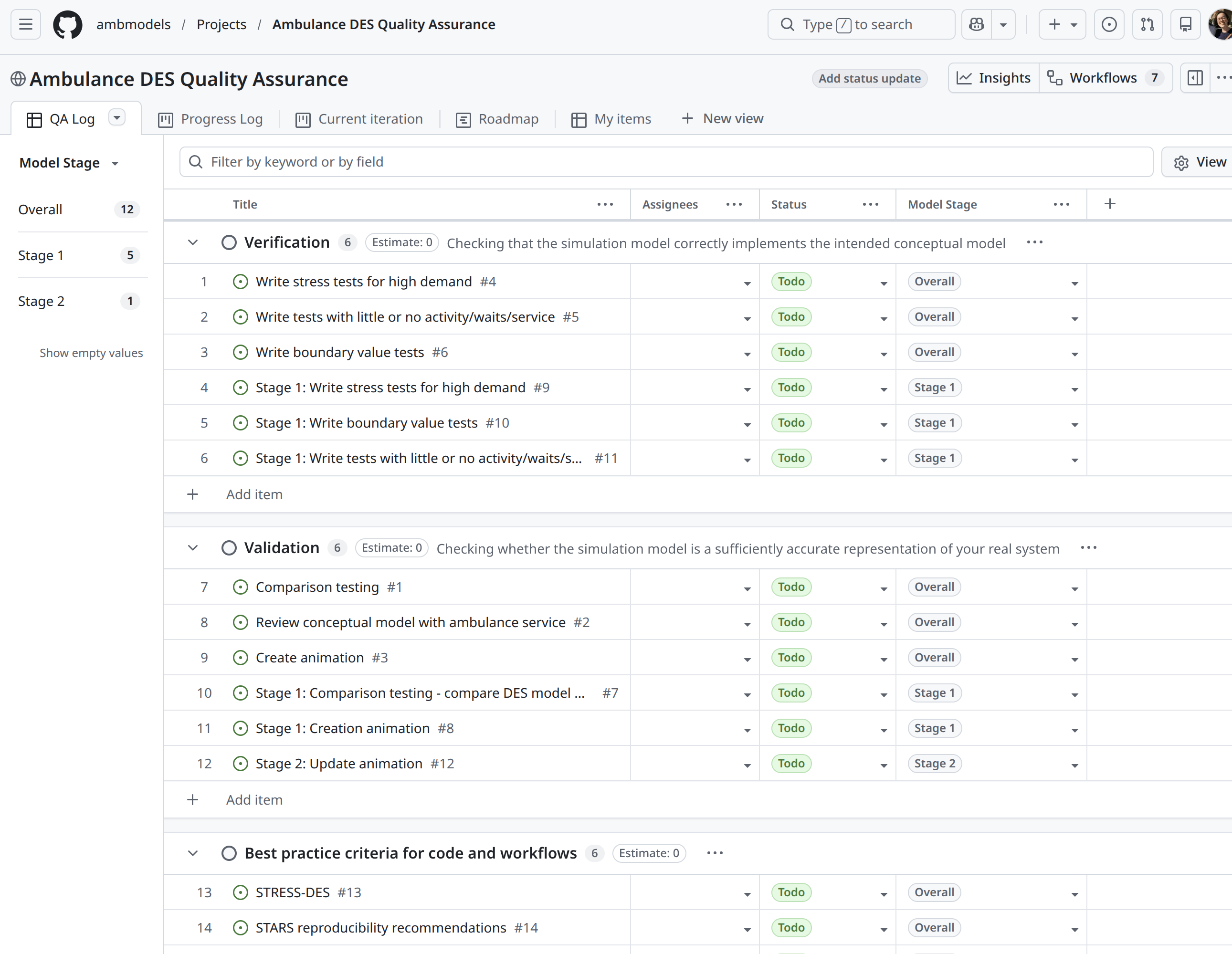](https://github.com/orgs/ambmodels/projects/1/views/1)
### Reuse
This model and the accompanying results were developed in partnership with the South Western Ambulance Service NHS Foundation Trust (SWASFT) for a specific service context, dataset and set of questions. They are shared to support transparency, learning and reuse of methods, but the results shown on this website should not be interpreted as directly applicable to other ambulance services, regions or operational settings without **further local adaptation and validation**.
## Reuse
We are keen for others to learn from and build on this work. The code is released under the MIT licence, so you are free to reuse, adapt and integrate it into your own projects, with attribution. We would be glad to hear from anyone interested in adapting the model for their own context.
However, it is important that any reuse involves appropriate local validation and does not simply apply the example results elsewhere. Anyone wishing to reuse this work should:
1. **Define the local purpose clearly** – what questions you want to answer, and what decisions the model is intended to inform in your setting.
2. **Review whether the structure matches your context** – check that the pathway, demand patterns, resources and performance measures in the code are appropriate for your service.
3. **Replace example data with local data** – use data from your own organisation, applying your local information governance and disclosure control rules.
4. **Repeat verification and validation locally** – work with your own stakeholders to check that the model behaves plausibly, reproduces key patterns in your data, and is suitable for the kinds of scenarios you want to explore.
If you are planning to adapt the model and would like to discuss this, please do get in touch.
## Citation
If you reuse this model, please cite us!
```{.txt}
{{< include ../../CITATION.cff >}}
```
## Knowledge for reuse
To make effective use of this model, some background knowledge may be helpful. You can find lots of relevant material in the [DES RAP Book](https://pythonhealthdatascience.github.io/des_rap_book/). At a minimum, we suggest:
* [**Discrete-event simulation**](https://pythonhealthdatascience.github.io/des_rap_book/pages/intros/des.html) - what DES is, how it represents systems, and why it is commonly used in healthcare modelling.
* [**Initialisation bias and warm-up periods**](https://pythonhealthdatascience.github.io/des_rap_book/pages/guide/output_analysis/warmup.html) - why simulation models can produce biased early results, and how warm-up periods help address this.
* [**Object-oriented programming (OOP)**](https://pythonhealthdatascience.github.io/des_rap_book/pages/guide/setup/code_structure.html) - useful background for understanding how the model code is structured.
### Validation
Validation is the process of checking whether the simulation model is a sufficiently accurate representation of your real system. It involves comparing the model's inputs, behaviour and results to the real system. The key question is whether any differences are small enough that the model can still reliably support the decisions or answer the questions it was designed for.
## Things I can definitely do
**Conceptual model validation**
* [ ] Document and justify all modeling assumptions.
* [ ] Review the conceptual model with people familiar with the real system to assess completeness and accuracy.
**Animation visualisation**
* [ ] Create an animation to help with validation (as well as communication and reuse).
**Cross validation**
* [ ] Search for similar simulation studies and compare the key assumptions, methods and results. Discuss discrepancies and explain reasons for different findings or approaches. Use insights from other studies to improve or validate your own model.
**Experimentation validation**
* [ ] Use a warm-up period.
* [ ] Use statistical methods to determine sufficient run length and number of replications.
* [ ] Perform sensitivity analysis to test how changes in input parameters affect outputs.
::: {.box-hl}
Good to discuss now **or later** what anticipate relevant to vary in sensitivity analysis.
:::
## Things that require data / processing from ambulance team
**Input data validation**
* [ ] Check the datasets used - screen for outliers, determine if they are correct, and if the reason for them occurring should be incorporated into the simulation.
* [ ] Ensure you have performed appropriate input modelling steps when choosing your distributions.
**Graphical comparison**
* [ ] Create time-series plots and distributions of key results (e.g., daily patient arrivals, resource utilisation, waiting times) for both the model and the actual system, and compare the graphs to assess whether patterns and trends are similar.
**Statistical comparison**
* [ ] Collect real system data on key performance measures (e.g., wait times, lengths of stay, throughput) and compare with model outputs statistically using appropriate tests.
**Predictive validation**
* [ ] Use historical arrival data, staffing schedules, treatment times, or other inputs from a specific time period to drive your simulation. Compare the simulation's predictions for that period (e.g., waiting times, bed occupancy) against the real outcomes for the same period.
* [ ] Consider varying the periods you validate on—year-by-year, season-by-season, or even for particular policy changes or events—to detect strengths or weaknesses in the model across different scenarios.
* [ ] Use graphical comparisons (e.g., time series plots) or statistical measures (e.g., goodness-of-fit, mean errors, confidence intervals) to assess how closely the model matches reality - see below.
::: {.box-hl}
**To discuss:**
* What would need to do these.
:::
## Other things we could consider doing
**Face validation**
* [ ] Present key simulation outputs and model behaviour to people such as: project team members; intended users of the model (e.g., healthcare analysts, managers); people familiar with the real system (e.g., clinicians, frontline staff, patient representatives). Ask for their subjective feedback on whether the model and results "look right". Discuss specific areas, such as whether performance measures (e.g., patient flow, wait times) match expectations under similar conditions.
**Turing test**
* [ ] Collect matching sets of model output and real system, remove identifying labels, and present them to a panel of experts. Record whether experts can distinguish simulation outputs from real data. Use their feedback on distinguishing features to further improve the simulation.
**Comparison testing**
* [ ] If you have multiple models of the same system, compare them!
*Can compare basic model to regression model. Requires some thought re: any other possible comparisons. we know of existing models and code and/or existing data. For example, could compare against and/or . Both open models. Or, could run with reported parameters of other models and compare. That's all alot of work though - depends if within capacity.*
::: {.box-hl}
**To discuss:**
* Whether we consider doing these.
:::
### Verification
Verification is the process of checking that the simulation model correctly implements the intended conceptual model. It involves checking that the model's logic, structure and parameters are implemented as planned and free from coding errors.
## Things I can definitely do
**Desk checking**
* [ ] Systematically check code.
* [ ] Keep documentation complete and up-to-date.
* [ ] Maintain an environment with all required packages.
* [ ] Lint code.
* [ ] Get code review
* Primarily using LLM - will provide code and prompt to review and identify any potential issues and improvements - we can then manually review
* Also, can explore other more occassional/one-off review from colleagues to check over (e.g., tests, docs, generally).
*
**Debugging**
* [ ] Write tests - they'll help for spotting bugs.
* [ ] During model development, monitor the model using logs - they'll help with spotting bugs.
* [ ] Use GitHub issues to record bugs as they arise, so they aren't forgotten and are recorded for future reference.
**Assertion checking**
* [ ] Add checks in the model which cause errors if something doesn't look right.
* [ ] Write tests which check that assertions hold true.
**Special input testing**
* [ ] If there are input variables with explicit limits, design boundary value tests to check the behaviour at, just inside, and just outside each boundary.
* [ ] Write stress tests which simulate worst-case load and ensure model is robust under heavy demand.
* [ ] Write tests with little or no activity/waits/service.
**Bottom-up testing**
* [ ] Write unit tests for each individual component of the model.
* [ ] Once individual parts work correctly, combine them and test how they interact - this can be via integration testing or functional testing.
**Regression testing**
* [ ] Write tests early.
* [ ] Run tests regularly (locally or automatically via. GitHub actions).
**Execution tracing**
* [ ] Trace individual calls or ambulances.
## Things that require some discussion
**Mathematical proof of correctness**
* [ ] For parts of the model where theoretical results exist (like an M/M/s queue), compare simulation outputs with results from mathematical formulas.
::: {.box-hl}
This **requires some thought** as to whether there is anything we could compare against for even the most basic model. To discuss with Tom. *Have put comparison to regression under comparison testing validation*
:::